Input data is specified in an input file.
Output is written to an info file
.
or
vctrans input
where input (or input.inp) denotes the input file. The input format uses, like all the Quantics package input files, keywords that are for the most part free format and case insensitive. See Quantics input file structure
vctrans input.inp
for further information on the general use of keywords, noting that there are no sections in the VCHAM input files. The input file ends with the keyword end-input
| Defining the system and input data files | |||||||||||||||||||||||||||
|---|---|---|---|---|---|---|---|---|---|---|---|---|---|---|---|---|---|---|---|---|---|---|---|---|---|---|---|
| Keyword | Description | ||||||||||||||||||||||||||
| file0 = S | S is name of file containing normal modes and Q0 geometry | ||||||||||||||||||||||||||
| nmodes = I (, I1) | System contains I normal modes and I1 trivial degrees
of freedom (default 6). |
||||||||||||||||||||||||||
| all_eigenvectors | Use all Hessian eigenvectors, including those corresponding to translations and infinitesimal rotations. NOT IN USE. |
||||||||||||||||||||||||||
| nstates = I | System contains I states. This needs to be the number included in the quantum chemistry calculations, i.e. the number of states in the output files. | ||||||||||||||||||||||||||
| Defining the point files to be read | |||||||||||||||||||||||||||
| Keyword | Argument | ||||||||||||||||||||||||||
| datadir = S | Files are contained in the directory S. Default is "." | ||||||||||||||||||||||||||
| files file.log I [options] .... end-files |
Read the data for state I from file.log. The files and end-files keywords must be alone on a line. Various options can be used
If I is given as 0, all state energies for a given point are read
|
||||||||||||||||||||||||||
| datasets data.set .... end-datasets |
Read the set of files listed in the file data.set. The
list uses the same format as the files ... end-files keywords. The datasets and end-datasets keywords must be alone on a line. |
||||||||||||||||||||||||||
| Defining the input data to be read from a GAUSSIAN output file. | |||||||||||||||||||||||||||
| abinitiotype = S |
Define the ab initio method used in the calculations to be
read
|
||||||||||||||||||||||||||
| Defining the input data to be read from a MOLPRO output file. | |||||||||||||||||||||||||||
| abinitiotype = S |
Define the ab initio method used in the calculations to be
read
|
||||||||||||||||||||||||||
| molpro_reorder | If states reorder between CAS and CAS-PT2 calculation this will read in derivative couplings and assign them to correct state. If used the CAS ordering of states must be given with the states keyword. The ordering of the states given in the info file is then written out in numerical order | ||||||||||||||||||||||||||
| Defining the input data to be read from a GAMMES-US output file. | |||||||||||||||||||||||||||
| abinitiotype = S |
Define the ab initio method used in the calculations to be
read
|
||||||||||||||||||||||||||
| Defining the input data to be read from a TURBOMOLE output file. | |||||||||||||||||||||||||||
| abinitiotype = S |
Define the ab initio method used in the calculations to be
read
|
||||||||||||||||||||||||||
| Defining the input data to be read from a DD-vMCG QC database. | |||||||||||||||||||||||||||
| abinitiotype = DB |
The database from a direct dynamics calculation will be transformed
into an info file for fitting. The following options must be set
in addition:
|
||||||||||||||||||||||||||
| DB0 | Only the first DB dataset is read and output. An analysis of the gradients and couplings will be made, ordering the modes in terms of coupling strengths. | ||||||||||||||||||||||||||
| file0abtype = S | S is the calculation type used for file0. If not
used, type is that defined by the abinitiotype keyword. See abinitiotype keyword above for options |
||||||||||||||||||||||||||
| gndabtype = S | If ground-state energies are read from separate files (see data file options above) S is the calculation type used in these files. See abinitiotype keyword above for options |
||||||||||||||||||||||||||
| order = I | I=0 only energies read at each point I=1 energies and gradients read if present in file Gradient Difference and Derivative coupling too. I=2 energies, gradients, and hessians read if present in file. |
||||||||||||||||||||||||||
| orient = S |
S is a string defining the input orientation to be read
|
||||||||||||||||||||||||||
| file0orient = S | Orientation to be read from file. This is used to select
the geometry in output from GAUSSIAN. See orient keyword for options. If not set, file0orient = orient |
||||||||||||||||||||||||||
| Defining the input data to be read from a MOLCAS output file. | |||||||||||||||||||||||||||
| abinitiotype = S |
Define the ab initio method used in the calculations to be
read
|
||||||||||||||||||||||||||
e.g. file0 = geometry0.log
will read the file geometry0.log for the information. If using
GAUSSIAN, this file should be created using the
freq=hpmodes keyword
| Defining the output | |
|---|---|
| Keyword | Argument |
| title line 1 .... end-title |
Add title to info file. The title keyword must be alone on a line and up to five lines can be written before the end-title keyword - which must also be alone on a line. |
| derivatives_in_q | If the first derivatives have been read for a dataset they are written out in normal mode coordinates as well as cartesian |
| second_derivatives_in_q | If the second derivatives (Hessian) have been read for a dataset they are written out in normal mode coordinates as well as cartesian |
| gradient_difference | If the derivative coupling and gradient difference are read for a dataset, both are written out. Otherwise only the derivative coupling is given. If derivative_in_q is also set these vectors are given in both cartesian and normal mode coordiantes |
| transition_dipoles | If the transition dipole moment between the ground-state and the state of interest has been read it is written out. |
| nmode_trafos | Output the cartesian to mass-frequency scaled normal mode transformation matrix. |
| units_au | Atomic units (Hartree and Bohr) used in place of the default eV and Angstrom. |
| Defining the system | |
|---|---|
| Keyword | Argument |
| energy0 = R | The zero of energy is taken as R. Input can can be in a variety of units |
| states = I, I1, ... | The database will include information from states I, I1, ... By convention I = 1 is the ground-state. E.g. states = 1,3,4 will read the ground-state, and the second- and third-excited states. If this keyword is not used, the database will read information for all states from 1,..., nstates as defined by the nstates keyword. |
| frequencies I LAB R .... end-frequencies |
for the Ith mode with label LAB use the frequency R instead of that read in the file0. Default is frequency in eV, but units can be used. |
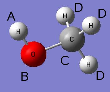
| nm2curv dihed = M | transforms the normal mode to the dihedral angle defined by the atoms in dihed-section (see note 1 below). |
The atom denoted a is not rotated but used as the reference for the dihedral angle. A is connected to b which forms part of the b-c bond which the dihedral angle is rotated about. The above digram would require the following example input section.
dihed-section
H a
O b
C c
H d
H d
H d
end-dihed-section
Any other atoms in the molecule which are not to be rotated and do not form part of the dihedral bond must be frozen using the flag f.
Is also worth mentioning that in the output database (.info) this normal mode will no longer be expressed in normal mode coordinates, but in torsional degrees.
The vibonic coupling model Hamiltonian has been
calculated for the lowest three states of Cr(CO)5. At
the D3h trigonal bipyramid geometry, these form an
(Exe)+A pseudo-Jahn-Teller system with a doubly degenerate state
coupled to a singly degenerate state. See Worth et al. Mol.
Phys. (2006) 104: 1095. In the fit the following 2
datadases of points were used.
crco5_trans0.info is
a zero-order info file for Cr(CO)5. It was created
using the input crco5_trans0.inp . According to this input,
the file CrCO5_D3h.log is the result of a GAUSSIAN
calculation containing the normal modes and frequencies. The
frequencies for the model, both for the mass-frequency scaled
coordinates and the zero-order Hamiltonian, are taken from the
input file rather than the GAUSSIAN calculation. The system
contains 27 normal modes. Information about the surfaces is read
up to second order (energy, first and second serivatives, and
gradient difference and derivative coupling) from the files
crco5_d3h_72.log and
crco5_d3h_73.log
which are both stored in the directory
points. The calculations have been done using a CAS
method, and the system will include information from for 3
states, labelled 1,2 and 3 in the files. Information about states
1 and 2 is read from crco5_d3h_72.log and information about state
3 is read from crco5_d3h_73.log. Energies in the .info
file are taken relative to -650.1354407439 and the
derivative coupling vectors, as well as the derivatives in the
dimensionless normal mode coordinate system are also written
out.
A second database was then set up with the energies of the
various states at a number of points along the most important
vibrational modes: crco5_trans1.info The input file was
crco5_trans1.inp . In contrast to the
crco5_trans0 the order is set to 0, which means
that only energies are read in. In addition to the files at
Q0 read before, the files listed in
crco5_1.set
crco5_2.set
crco5_8.set
are to be read.
These are the points along modes 1, 2, and 8
respectively.